Extend scikit-learn FastICA example to use Icasso

FastICA is fit multiple times to simple example data and performance can be visually inspected.

# Authors: Erkka Heinila <erkka.heinila@jyu.fi>
#
# License BSD (3-clause)

from itertools import cycle

import numpy as np
import matplotlib.pyplot as plt

from scipy import signal

from sklearn.decomposition import FastICA
from sklearn.decomposition import PCA

from icasso import Icasso

For replicability

random_state = 50
distance=0.12

Generate sample data

n_samples = 2000
time = np.linspace(0, 8, n_samples)

s1 = np.sin(2 * time)  # Signal 1 : sinusoidal signal
s2 = np.sign(np.sin(3 * time))  # Signal 2 : square signal
s3 = signal.sawtooth(2 * np.pi * time)  # Signal 3: saw tooth signal

S = np.c_[s1, s2, s3]

Add noise and standardize

S += 0.4 * np.random.RandomState(random_state).normal(size=S.shape)
S /= S.std(axis=0)

Mix data

A = np.array([[1, 1, 1], [0.5, 2, 1.0], [1.5, 1.0, 2.0]])
X = np.dot(S, A.T)

Define functions for extracting bootstraps and unmixing matrices from ica object

def bootstrap_fun(data, generator):
    return data[generator.choice(range(data.shape[0]), size=data.shape[0]), :]

def unmixing_fun(ica):
    return ica.components_

Create the Icasso object

ica_params = {
    'n_components': 3
}
icasso = Icasso(FastICA, ica_params=ica_params, iterations=100, bootstrap=True,
                vary_init=True)

Fit the Icasso

icasso.fit(data=X, fit_params={}, random_state=random_state,
           bootstrap_fun=bootstrap_fun, unmixing_fun=unmixing_fun)

Plot dendrogram

icasso.plot_dendrogram()

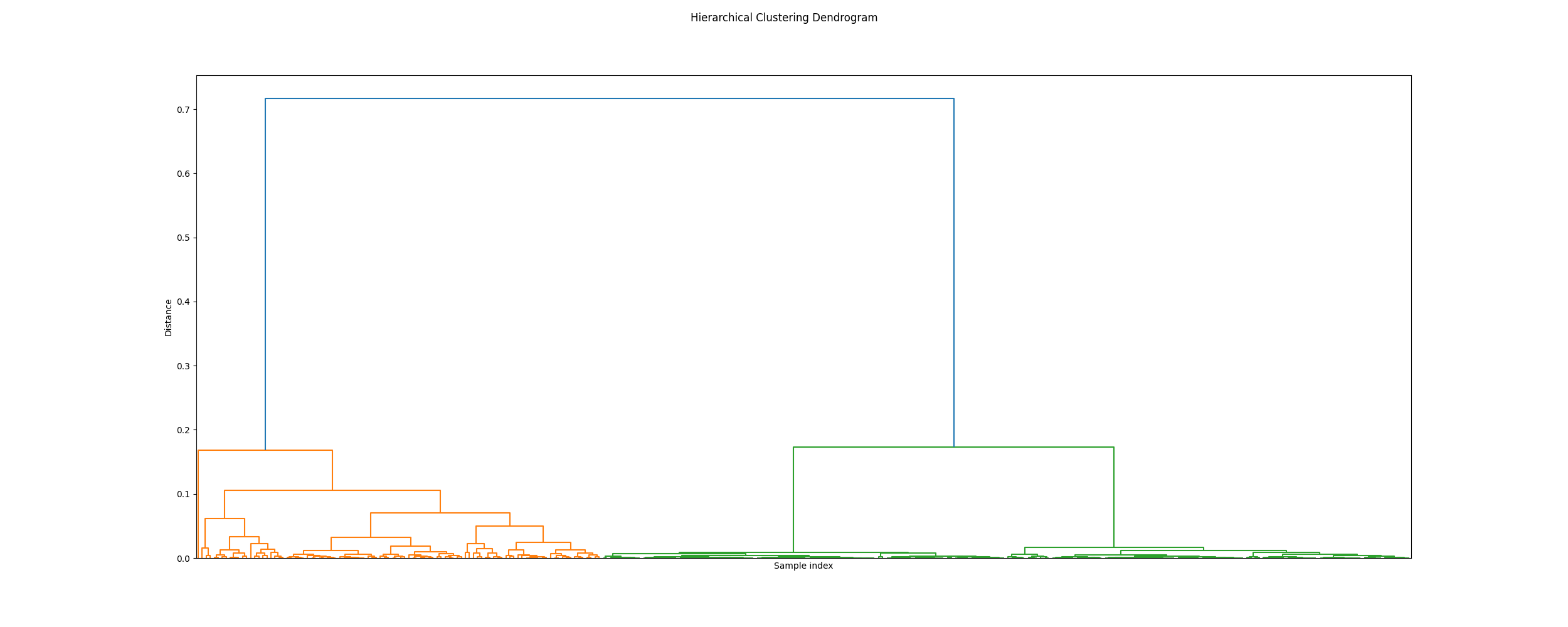
Out:

<Figure size 2500x1000 with 1 Axes>

Plot mds

icasso.plot_mds(distance=distance)

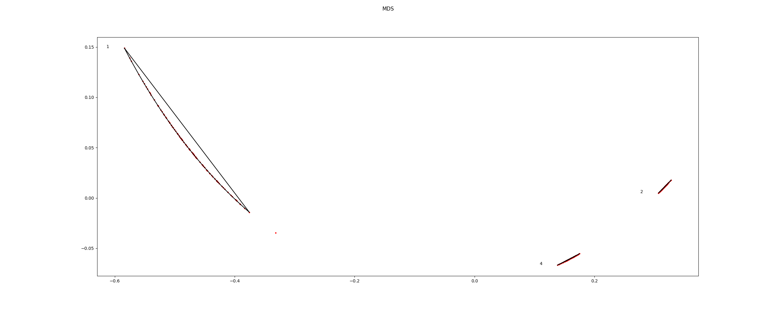
Out:

<Figure size 2500x1000 with 1 Axes>

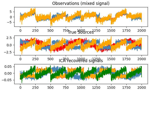
Get the unmixing matrix and use it get the sources.

W_, scores = icasso.get_centrotype_unmixing(distance=distance)
S_ = np.dot(W_, X.T).T

# #############################################################################
# Plot results
plt.figure()

models = [X, S, S_,]
names = ['Observations (mixed signal)',
         'True Sources',
         'ICA recovered signals']

for ii, (model, name) in enumerate(zip(models, names), 1):
    colors = cycle(['red', 'steelblue', 'orange', 'green', 'yellow'])
    plt.subplot(4, 1, ii)
    plt.title(name)
    for sig, color in zip(model.T, colors):
        plt.plot(sig, color=color)

plt.subplots_adjust(0.09, 0.04, 0.94, 0.94, 0.26, 0.46)
plt.show()