Use Icasso to compute and validate ICA on MEG data

ICA is fit to MEG raw data multiple times, and the performance is then visually inspected. Finally the components are retrieved as centrotypes of the most robust clusters.

# Authors: Erkka Heinila <erkka.heinila@jyu.fi>
#
# License: BSD (3-clause)

import logging

import numpy as np
import matplotlib.pyplot as plt
import mne

from mne.preprocessing import ICA
from mne.preprocessing import create_ecg_epochs, create_eog_epochs
from mne.datasets import sample

from icasso import Icasso

Set up logging

logging.basicConfig(level=logging.INFO)

Setup paths and prepare raw data.

data_path = sample.data_path()
raw_fname = data_path + '/MEG/sample/sample_audvis_filt-0-40_raw.fif'

raw = mne.io.read_raw_fif(raw_fname, preload=True)
raw.filter(1, None, fir_design='firwin')

picks = mne.pick_types(raw.info, meg='grad', eeg=False, eog=False,
                       stim=False, exclude='bads')
raw.drop_channels([ch_name for idx, ch_name in enumerate(raw.info['ch_names'])
                   if idx not in picks])

Out:

/home/erpipehe/Code/Teekuningas/icasso/examples/plot_icasso_from_raw.py:32: DeprecationWarning: data_path functions now return pathlib.Path objects which do not natively support the plus (+) operator, switch to using forward slash (/) instead. Support for plus will be removed in 1.2.
  raw_fname = data_path + '/MEG/sample/sample_audvis_filt-0-40_raw.fif'
Opening raw data file /home/erpipehe/mne_data/MNE-sample-data//MEG/sample/sample_audvis_filt-0-40_raw.fif...
    Read a total of 4 projection items:
        PCA-v1 (1 x 102)  idle
        PCA-v2 (1 x 102)  idle
        PCA-v3 (1 x 102)  idle
        Average EEG reference (1 x 60)  idle
    Range : 6450 ... 48149 =     42.956 ...   320.665 secs
Ready.
Reading 0 ... 41699  =      0.000 ...   277.709 secs...
Filtering raw data in 1 contiguous segment
Setting up high-pass filter at 1 Hz

FIR filter parameters
---------------------
Designing a one-pass, zero-phase, non-causal highpass filter:
- Windowed time-domain design (firwin) method
- Hamming window with 0.0194 passband ripple and 53 dB stopband attenuation
- Lower passband edge: 1.00
- Lower transition bandwidth: 1.00 Hz (-6 dB cutoff frequency: 0.50 Hz)
- Filter length: 497 samples (3.310 sec)

Removing projector <Projection | PCA-v1, active : False, n_channels : 102>
Removing projector <Projection | PCA-v2, active : False, n_channels : 102>
Removing projector <Projection | PCA-v3, active : False, n_channels : 102>
Removing projector <Projection | Average EEG reference, active : False, n_channels : 60>

Measurement date	December 03, 2002 19:01:10 GMT
Experimenter	Unknown
Participant	Unknown
Digitized points	0 points
Good channels	203 Gradiometers
Bad channels	None
EOG channels	Not available
ECG channels	Not available
Sampling frequency	150.15 Hz
Highpass	1.00 Hz
Lowpass	40.00 Hz
Filenames	sample_audvis_filt-0-40_raw.fif
Duration	00:04:37 (HH:MM:SS)

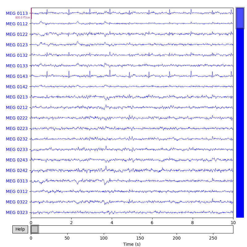
Plot raw data

raw.plot(block=True)

Out:

Using matplotlib as 2D backend.
Opening raw-browser...

<MNEBrowseFigure size 800x800 with 4 Axes>

Define parameters for mne’s ICA-object and create a Icasso object. Set bootstrap=True to use bootstrapping.

ica_params = {
    'n_components':20,
    'method': 'fastica',
    'max_iter': 1000,
}
icasso = Icasso(ICA, ica_params=ica_params, iterations=30,
                bootstrap=False, vary_init=True)

Set up params for ICA.fit method.

fit_params = {
    'decim': 3,
    'verbose': 'warning'
}

Set up function for getting bootstrapped versions of Raw object.

def bootstrap_fun(raw, generator):
    sample_idxs = generator.choice(range(raw._data.shape[1]), size=raw._data.shape[1])
    raw = raw.copy()
    raw._data = raw._data[:, sample_idxs]
    return raw

Set up function to get unmixing matrix from mne’s ICA object after fitting.

def unmixing_fun(ica):
    unmixing_matrix = np.dot(ica.unmixing_matrix_,
                             ica.pca_components_[:ica.n_components_])
    return unmixing_matrix

Set up function to store information about individual runs. We do this to get pca mean and pre_whiten information.

def store_fun(ica):
    data = {'pre_whitener': ica.pre_whitener_,
            'pca_mean': ica.pca_mean_[:, np.newaxis]}
    return data

For replicability

random_state = 10
distance = 0.75

Fit icasso to raw data.

icasso.fit(data=raw, fit_params=fit_params, random_state=random_state,
           bootstrap_fun=bootstrap_fun, unmixing_fun=unmixing_fun,
           store_fun=store_fun)

Out:

INFO:icasso:Fitting ICA 30 times.

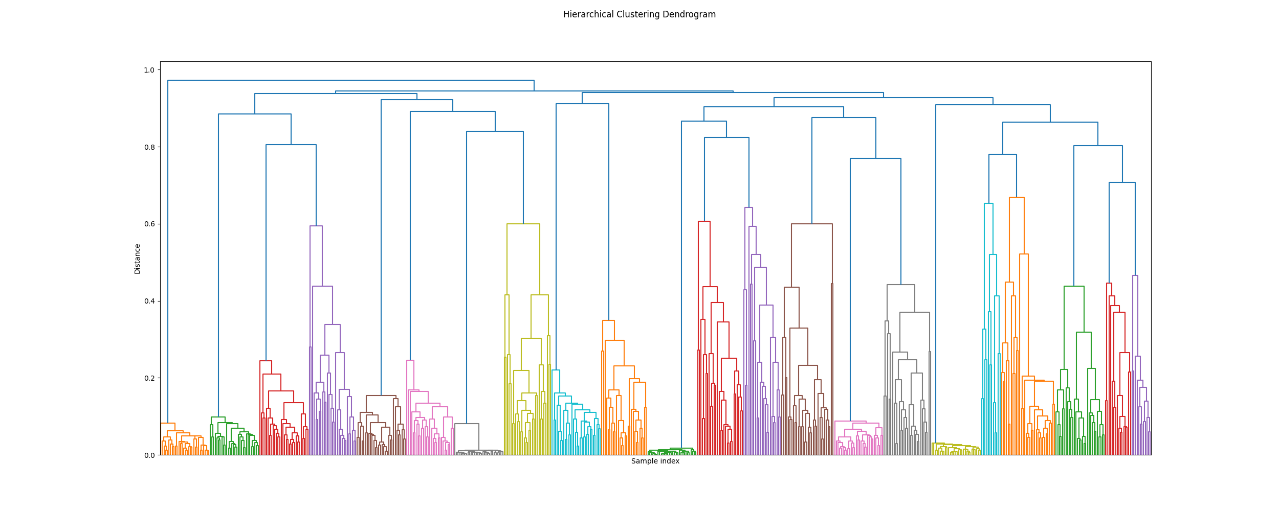
Plot a dendogram

icasso.plot_dendrogram()

Out:

INFO:icasso:Plotting dendrogram..

<Figure size 2500x1000 with 1 Axes>

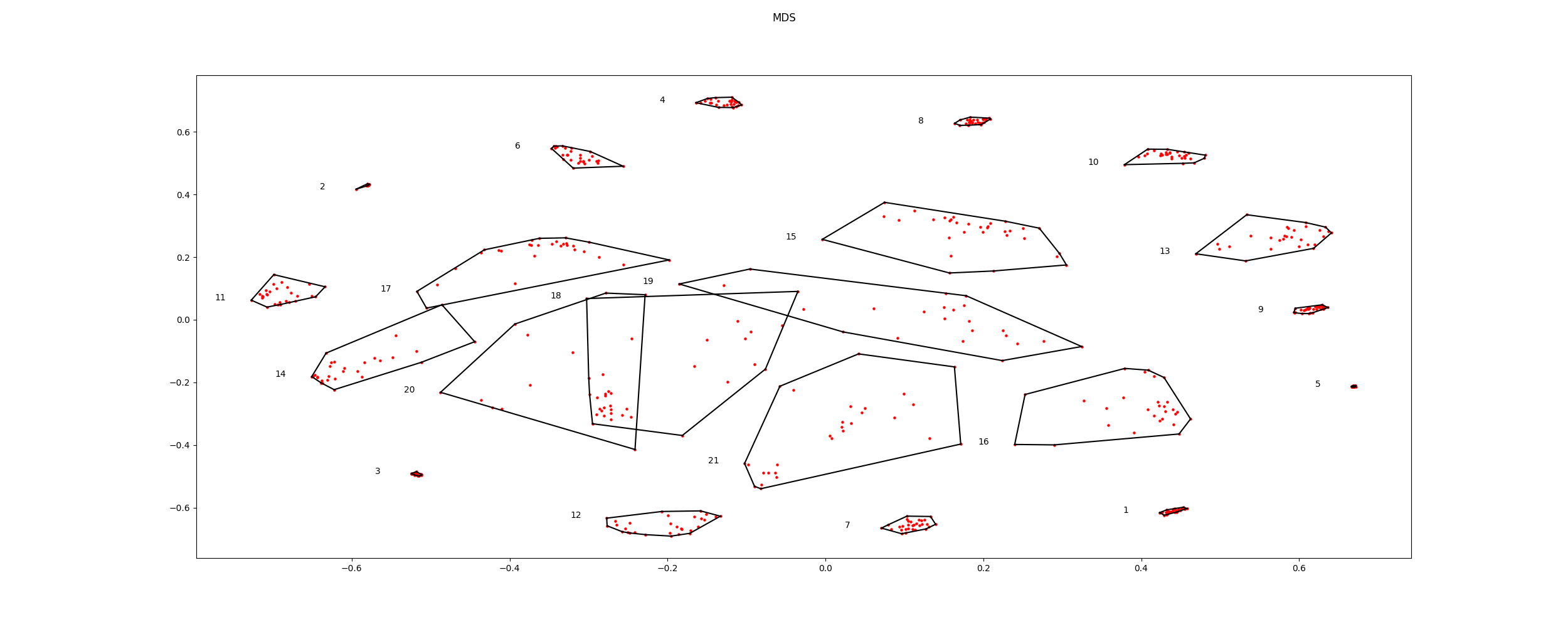
Plot the components in 2D space.

icasso.plot_mds(distance=distance)

Out:

INFO:icasso:Projecting components to 2D space with MDS
INFO:icasso:Plotting ICA components in 2D space..

<Figure size 2500x1000 with 1 Axes>

Unmix using the centrotypes

unmixing, scores = icasso.get_centrotype_unmixing(distance=distance)
pca_mean, pre_whitener = icasso.store[0]['pca_mean'], icasso.store[0]['pre_whitener']
sources = np.dot(unmixing, (raw._data / pre_whitener) - pca_mean)

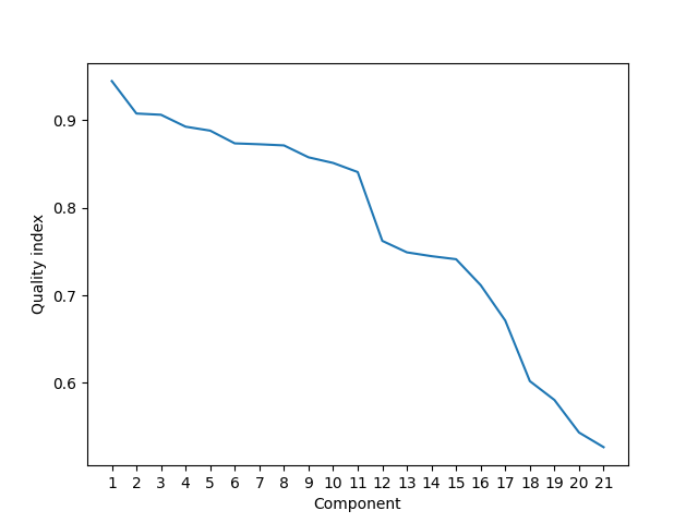
Show cluster quality indices.

plt.figure()
plt.plot(range(1, len(scores)+1), scores)
plt.xticks(range(1, len(scores)+1),
           [str(idx) for idx in range(1, len(scores)+1)])
plt.xlabel('Component')
plt.ylabel('Quality index')
plt.show()

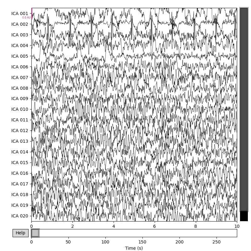
Create raw object using the icasso centrotype sources and plot it

sources = sources * 3e-04
info = mne.create_info(['ICA %03d' % (idx+1) for idx in range(sources.shape[0])],
                       raw.info['sfreq'], ch_types='misc')
components = mne.io.RawArray(sources, info)
components.plot(block=True)

Out:

Creating RawArray with float64 data, n_channels=21, n_times=41700
    Range : 0 ... 41699 =      0.000 ...   277.709 secs
Ready.
Opening raw-browser...

<MNEBrowseFigure size 800x800 with 4 Axes>